What is Regularization?
In a general manner, to make things regular or acceptable is what we mean by the term regularization. This is exactly why we use it for applied machine learning. In the domain of machine learning, regularization is the process which prevents overfitting by discouraging developers learning a more complex or flexible model, and finally, which regularizes or shrinks the coefficients towards zero. The basic idea is to penalize the complex models i.e. adding a complexity term in such a way that it tends to give a bigger loss for evaluating complex models.
In other words, a form of predictive modelling technique which investigates the relationship between a target variable to its predictor i.e., the independent variable is what we know as regression analysis. Mostly, this technique is used for forecasting, time series modelling and finding the causal effect relationship between the variables. A real-time example is the relationship between prediction of salary of new employees depending on years of work experience is best studied through regression.
Now, the next question arises is why do we use Regression Analysis?
Regression analysis provide us the easiest technique to compare the effects of variables measured on different range, such as the effect of salary changes and the number of upcoming, promotional activities. These benefits help market researchers’, data analysts’ and data scientists to eliminate and evaluate the best set of variables to be used for building predictive models.
As already discussed above, regression analysis helps to estimate the relationship between dependent and independent variables. Let’s understand this with an easy example:
Suppose we want to estimate the growth in sales of a company based on current economic conditions of our country. The recent company data available with us speaks that the growth in sales is around two and a half times the growth in the economy.
Using the regression insight, we can easily predict future sales of the company based on present & past information. There are multiple benefits of using regression analysis. They are as such as it provides a prediction by indicating the significant relationships between dependent variable and independent variable and depicting the strength of impact of multiple independent variables on a dependent variable.
Now, moving on with the next important part on what are the Regularization Techniques in Machine Learning.
Regularization Techniques
There are mainly two types of regularization techniques, namely Ridge Regression and Lasso Regression. The way they assign a penalty to β (coefficients) is what differentiates them from each other.
Ridge Regression (L2 Regularization)
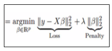
This technique performs L2 regularization. The main algorithm behind this is to modify the RSS by adding the penalty which is equivalent to the square of the magnitude of coefficients. However, it is considered to be a technique used when the info suffers from multicollinearity (independent variables are highly correlated). In multicollinearity, albeit the smallest amount squares estimates (OLS) are unbiased, their variances are large which deviates the observed value faraway from truth value. By adding a degree of bias to the regression estimates, ridge regression reduces the quality errors. It tends to solve the multicollinearity problem through shrinkage parameter λ. Now, let us have a look at the equation below.
In this equation, we have two components. The foremost one denotes the least square term and later one is lambda of the summation of β2 (beta- square) where β is the coefficient. This is added to least square term so as to shrink the parameter to possess a really low variance.
Every technique has some pros and cons, so as Ridge regression. It decreases the complexity of a model but does not reduce the number of variables since it never leads to a coefficient tending to zero rather only minimizes it. Hence, this model is not a good fit for feature reduction.
Lasso Regression (L1 Regularization)
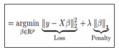
This regularization technique performs L1 regularization. Unlike Ridge Regression, it modifies the RSS by adding the penalty (shrinkage quantity) equivalent to the sum of the absolute value of coefficients.
Looking at the equation below, we can observe that similar to Ridge Regression, Lasso (Least Absolute Shrinkage and Selection Operator) also penalizes the absolute size of the regression coefficients. In addition to this, it is quite capable of reducing the variability and improving the accuracy of linear regression models.
Limitation of Lasso Regression:
- If the number of predictors (p) is greater than the number of observations (n), Lasso will pick at most n predictors as non-zero, even if all predictors are relevant (or may be used in the test set). In such cases, Lasso sometimes really has to struggle with such types of data.
- If there are two or more highly collinear variables, then LASSO regression select one of them randomly which is not good for the interpretation of data.
Lasso regression differs from ridge regression in a way that it uses absolute values within the penalty function, rather than that of squares. This leads to penalizing (or equivalently constraining the sum of the absolute values of the estimates) values which causes some of the parameter estimates to turn out exactly zero. The more penalty is applied, the more the estimates get shrunk towards absolute zero. This helps to variable selection out of given range of n variables.
Practical Implementation of L1 & L2 Using Python
Now, let’s have a practical experience of ridge and lasso regression implementation in python programming language.
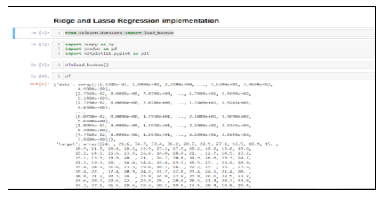
As like any other project, we import our usual libraries that will help us perform basic data manipulation and plotting. And then, we start off by importing our dataset and looking at its rows and columns.
The problem that we will try to solve here is that given a set of features that describe a house in Boston, our machine learning model must predict the house price.
At the very outmost, we will be importing the Boston dataset and display its data frame contents.
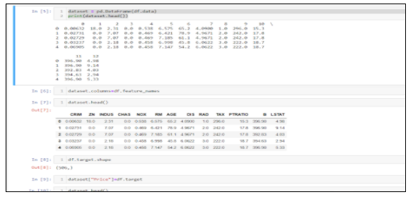
The very next step is to visualize the data frame rows and columns which is known an Exploratory Data Analysis. The Boston data frame has 506 rows and 14 columns containing the columns: crim, zn, indus, chas, nox, rm, age, dis, rad, tax, ptratio, black, lstat and medv.
Now, we shall find the mean squared error using Linear Regression, Ridge Regression and Lasso Regression and try to find out which gives us the best result.
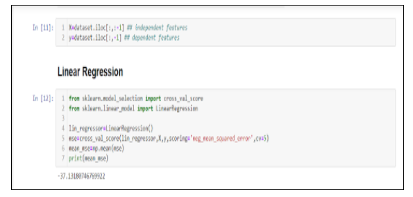
First, we import the Linear Regression and cross_val_score objects. The first one will allow us to fit a linear model, while the second object will perform k-fold cross-validation. Then, we define our features and target variable. The cross_val_score will return an array of MSE for each cross-validation steps. In our case, we have five of them. Therefore, we take the mean of MSE and print it. We are getting a negative MSE of -37.1318.
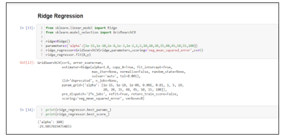
Now, let’s see if ridge regression works better or lasso will be better. For ridge regression, we introduce GridSearchCV. This will allow us to automatically perform 5-fold cross-validation with a range of different regularization parameters in order to find the optimal value of alpha. You should see that the optimal value of alpha is 100, with a negative MSE of -29.90570. We can easily observe a slight improvement on comparing with the basic multiple linear regression.
The code looks like this:
Lasso
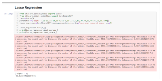
As ridge regression, the same process is followed for lasso. In this case, the optimal value for alpha is 1, and the negative MSE is -35.5315, which is the best score of all three models!
The Conclusion…
Hope this article has given you all a brief idea on Regularization, the types of techniques namely Ridge and Lasso Regression, their pros and cons and finally, implementation with the help of Python.


